Commands: emegs2d
Contents:
Loading data: To open the standard display of
an evoked signal, type emegs2d
and hit return. On the
emegs2d command window, select your data format in the file menu at
\File\Data format. The default format is SCADS (meaning Statistical Control of Artifacts in Dense array Systems), which is the
format in
which data is saved during averaging in EmegsAVG. Files of this format
most often are named *.at* or *.at*.ar (if an average reference
was applied). Hit the 'Open Data
Set'-button and select a SCADS-file to load. Emegs then reads the data
file and retrieves the corresponding sensor
configuration as described on the ![]() sensor-configuration page.
Sensor positions are projected onto a plane, so that they look as seen
from above but flattened to the sides with the top of the data window
beeing anterior, the bottom posterior, left window border left side of
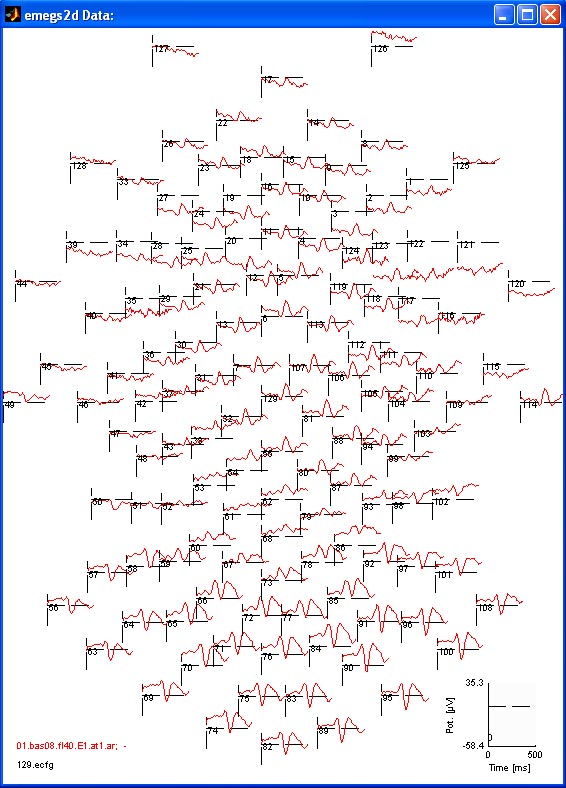
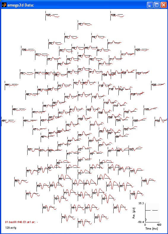
the head and right window border right side of the head. The example
below shows again an evoked scalp potential of an EGI 129 channel
device. [
sensor-configuration page.
Sensor positions are projected onto a plane, so that they look as seen
from above but flattened to the sides with the top of the data window
beeing anterior, the bottom posterior, left window border left side of
the head and right window border right side of the head. The example
below shows again an evoked scalp potential of an EGI 129 channel
device. [![]() Top]
Top]
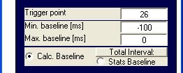
Baseline correction: in most cases, evoked activity needs to be baseline corrected. Again most of the times, an interval before stimulus onset (the trigger point) is used for that purpose. When loaded however, baseline correction is not active and must be activated manually. If you also want timing to be relative to a trigger point other the then first data point of the evoked signal, enter a point number in the trigger point edit box. Emegs then automatically sets Min. baseline [ms] to the length of all points before this point (e.g. if with a sampling rate of 250Hz you enter a trigger point of 26, min. baseline will be -100 ms) and Max. baseline [ms] to 0, thus selecting all points before the triggerpoint for baselinecorrection. The baseline then can be activated with the given settings by activating the Calc. Baseline - radiobutton.
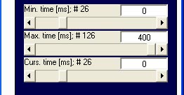
Note that setting the trigger
point will alter also the values in the min-, max- und cursortime
controls: possible values now range from -100 to 400ms whereas before
the range was 0 to 500 ms.
The curves are thus drawn to the zero line. Moreover the baseline
interval now is now hidden, as Min.
time [ms] is set to 0, which corresponds the 26th data
point: [![]() Top]
Top]
Zooming a sensor: To display
on selected channel separately, you can select a channel number
from the Zoom sensor-dropdownlist.

Two new windows will open, one displaying the data, and one to control
the data display of the channel. An example of channel 76 is given
below:
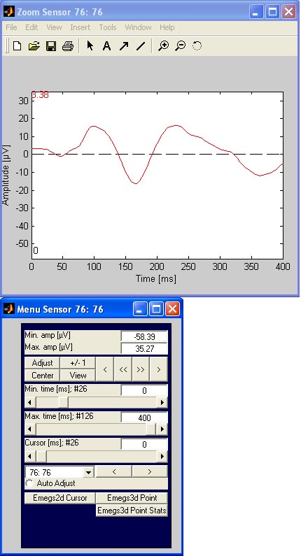
The menu window can be used for adjusting the amplitude scaling, and
choosing the timing limits. Zooming can also be done by activating
mouse zoom with the mouse-button
underneath the Zoom sensor-dropdownlist.
If activated, clicking on an axis on the data window will zoom to the
channel that you clicked on. If you wish to jump through multiple
channels, this will open a lot of windows. To prevent this, you can
push update on the right of
the mouse-button, to display
each new zoomed channel in the same windows, rather than opening new
windows for each channel. Push mouse or
update again to deactivate the
corresponding behavior. [![]() Top]
Top]
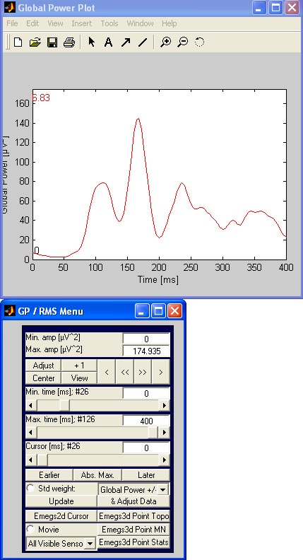
Global Power (GP) / Root mean square (RMS):
One way of identifying time ranges of great activity in an evoked
signal is to calculate the so called global power. This corresponds the
average of all squared channel waveforms, resulting in only one wave,
with big amplitudes indicating large amplitudes on many sensors. If you
want to get a realistic impression of the actual amplitudes, one can
calculate the square root of the global power - the result is called Root mean square.
To do either calculation with emegs, push the GP / RMS - button.

Two new windows will open similar to the zoom sensor windows, one of
which contains the data, and the other offering controls for the
scaling, timing and calculation type:
[![]() Top]
Top]
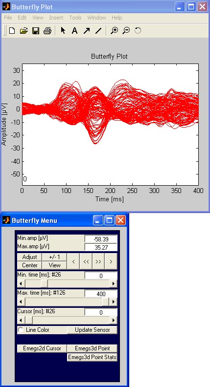
Butterfly plot: To creat an overlayed plot
of all channels, hit the butterfly-button.
This will again open a data and a command window as shown below: [![]() Top]
Top]
continuous data (Egis Continous &
EDF/BDF Raw):
continous data display serves to show the unprocessed raw data as
recorded during an experiment. Channels are arranged as a list,
ignoring spherical coordinates. This display type can be helpful for
visually identifying artefactual channels, finding blinks or checking
presented triggers. When switching to Egis
Continuous or EDF/BDF
Raw file format, the emegs2d-menu is changed a little to
include slidercontrols for the number and vertical position of
displayed channels, as shown below. The number of visible channels
determine how many channels are shown on the data window at a time, the
vertical position sets the number of the first (topmost) channel to
display.
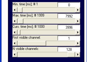
You can navigate back and forth in the data file using the cursor
time slider. Trigger values are plotted topmost in emegs2d data window.
An example of a 128 channel recording is shown below. Note that
BDF data is baseline corrected over the entire displayed interval to
allow equal scaling across channels despite DC offsets. [![]() Top]
Top]

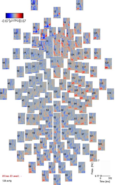
wavelet data: wavelet data differs from
standard ERPs/ERFs most importantly in the respect, that it contains
more information per sensor: not only one activity signal (or vector)
is given, but one signal for each frequency in the spectrum (a data
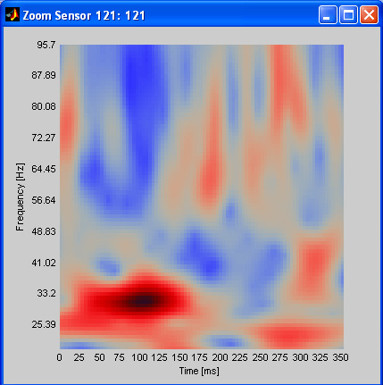
matrix). This matrix can be displayed as spectrogram, with color coded
amplitude (power). An example is shown below, with reddish
colours coding higher and blueish colours coding lower spectral power.
A clear activity maximum is visible around 100 ms and 30 Hz.
Emegs wavelet data is stored in files ending on .awa or .pwa. To
load wavelet data in emegs2d, first select the corresponding data
format from the file menu: \file\Data Format\Wavelet Amplitude (for
*.awa-files) or \file\Data Format\Wavelet Phaselock (for
*.pwa-files). Second, hit the open Open
Data Set-button and select your datafile. An additional
frequency selection window opens, and data is displayed in emegs2d data
window. Initially data is displayed as normal signals (lines, not
matrices) that correspond the averaged spectral power response over the
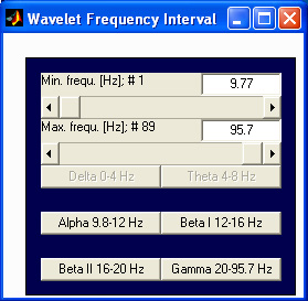
selected frequency range. The frequency range to be averaged can
be selected on the additional frequency selection window, that is shown
below:
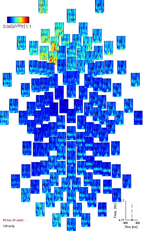
To display spectrograms as the one shown above instead of the
averaged power responses, select the domain Amp. W. II from the domain dropdownlist:

Your data window then should look something like this:
You can subtract a baseline just as for standard ERPs, using the
trigger point, min. baseline max. baseline and calc. baseline controls.
The only difference is that baseline correction is performed separately
per frequency, levelling overall power differences between bands. You
can adjust the colormap used for the spectrograms by selecting a
different colormap from emegs2d-style-menu (\Style\Wavelet\Colormap\).
The example shown below is baseline corrected and uses the galaxy
colormap. By using the center-button
you adjust the amplitude scaling, such that spectral powers at baseline
level are displayed with the color at the exact middle of the current
colormap (gray for galaxy). Especially for 3- or 4-colour-type
colormaps (like jet, galaxy or sahara), this is useful for quickly
discerning power increases and decreases, relative to baseline
levels. [![]() Top]
Top]
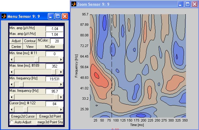
wavelet data: zooming a sensor
To zoom a sensor of the spectrogram display, simly click on the
spectrogram. A new window will open as for the standard sensor zoom,
except that the menu also allows you to set the frequency range and the
plot type. You can select the standard image plot type, or a contour
plot type that is shown below. The number of colors (contourlines) can
be entered on the menu as well. [![]() Top]
Top]
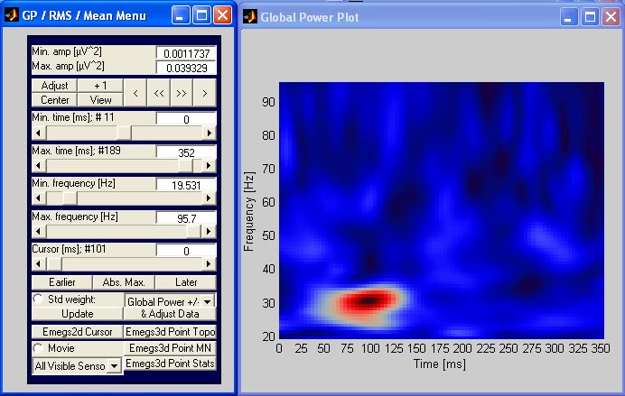
wavelet data: global power
the global power for wavelet data is activated using the global
power-button on emegs2d menu. A sample plot is shown below. [![]() Top]
Top]
volume data: volume data display in emegs
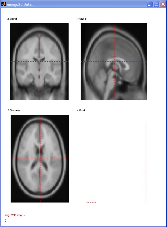
shows sagittal, coronal and transverse view analog to the display type
in MRICro. Select MRI analyze as
data format and select an img/hdr filepair. The emegs2d-menu is changed a little to
provide sliders for settings the sagittal, coronal and transverse slice:
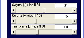
You can navigate in the volume
using the slider or by mouseclick on the displayed slices in the data
window. The current complementary slice planes are shown as red lines
on each view. You can adjust the black and white scaling using the
standard Min. Amp. and Max. Amp. editboxes. [![]() Top]
Top]
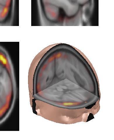
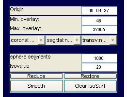
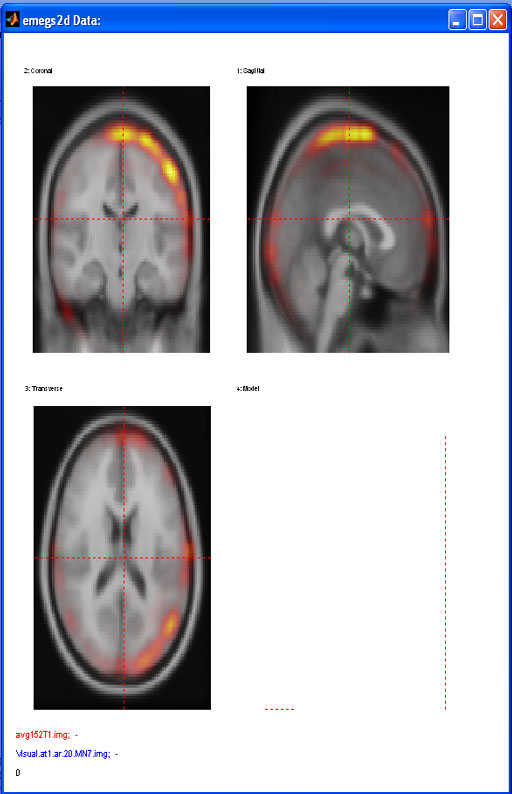
volume data: functional overlay: to load and display a functional overlay on a loaded image, select active data set number 2 and open the overlay img/hdr. Note that at the present point, image and overlay must be of equal size and origin to be displayed correctly. You can adjust the scaling of the overlay coloring using the Min. overlay and Max. overlay controls on emegs2d menu shown below :
The default colormap for the overlay is hot, but you can change the colormap
for both the base image and for the overlay separately using the
emegs2d-menu items \Style\MRI\Colormap
image and \Style\MRI\Colormap
overlay. An example with default colormap settings is shown
below. [![]() Top]
Top]
volume data: isosurface plots:
isosurface plots can be activated
using the 3 dropdownmenus below the Overlay scaling controls: for each
slice plane you can select a side that will be plotted - left or right
for the sagittal, top or down for the transverse and anterior or
posterior for the coronal axes. The other half will be removed, the
resulting volume will outline a volume above the IsoValue given in the IsoValue
editbox, and will be capped with a coloured slice plane in the model
axes. Using all three slice planes consequtively, you can thus create a
cut-out volume effect, as shown in the example below. Clear the model
axes using the Clear IsoSurf-button.
